Advanced Data Analysis Method
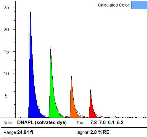
Dakota’s proprietary Advanced Data Analysis (ADA) software (written in Matlab) allows the Dakota analyst to “harvest” waveforms from field logs or bench-top tests and place them in the Basis Set and assign them proper names. Once the Basis Set has been properly populated, the LIF logs are individually loaded into the ADA software and a unique Background waveform is selected, usually from a depth that is yielding the lowest response. In rare cases, no background waveforms are possible due to a “top-to-bottom” LIF fluorescence response that never seems to reach low background intensities. In those cases a neighboring log’s Background is used or the Background is left out of the analysis.
Once the analyst is satisfied with the “setup” the ADA software automatically compares the Basis Set waveforms to all of the log’s raw waveforms (all the depths). The ADA software accomplishes this by passing each raw waveform, along with the Basis Set waveforms, to Matlab’s non-negative least squares (NNLS) fitting routine. This NNLS routine determines the proportion of each of the Basis Set waveforms that is required to optimally fit the raw waveform and returns a non-negative contribution for each Basis waveform for each depth in the log. Once the entire log of waveforms has been analyzed, the ADA software plots the original “raw” LIF log, the logs that represent the %RE that was mathematically attributable to each of Basis Set waveforms.
In addition to the Basis Set logs the ADA software also calculates the Residual log which is the sum of any mismatch between the synthetic waveform generated by the NNLS analysis and the raw waveform. Large residuals (relative to the original log) will result when the Basis Set does not contain waveforms similar to those encountered in the log because no matter what combination of “inappropriate” Basis Set waveforms it tries to combine, it won’t result in a waveform that assumes the same shape as the raw waveform. Large residuals are an indicator that either the Basis Set needs additional or different waveforms than those selected or that there has been saturation of the fluorescence detection system resulting in distorted raw waveforms (common on the first encounter of LNAPL with depth). Small residuals (relative to the raw fluorescence values) are an indicator that the Basis Set contained the waveforms necessary to properly fit the raw data and no Basis Set re-optimization is necessary.
 Classification or “Scatter” Plots
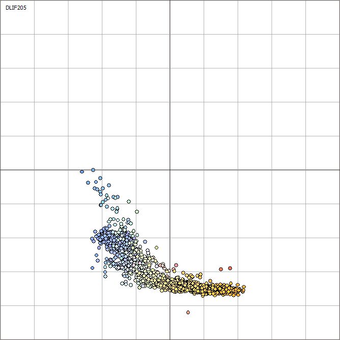
The amount of data in LIF can be overwhelming. With classification plots information from the hundreds (or even thousands) of waveforms from a single LIF log are “condensed” and then plotted on a 2D surface as color-coded spheres, allowing a spatial method of grouping or identifying clusters of fluorescence waveforms. Below is a description of characteristic classification plots and examples of how to interpret them.
X-Axis: Wavelength
In general terms the “center of mass” of the curve that is the fluorescence waveform determines the x-axis position on the classification plot for each sphere that represents a waveform. For example, a waveform that is dominated by a large blue peak plots far to the left on the x-axis, while a waveform dominated by the red peak plots far to the right on the x-axis.
 Y-Axis: Lifetime
The lifetime (decay of fluorescence over time) of the waveform’s four peaks (described in crude terms as the “width” of the peaks at 1/3 their maximum height) determines the y-axis position of the log data spheres. Short lifetimes (near zero “skinny” peaks) are plotted very low on the y-axis. The longer the lifetimes of the four peaks get (i.e. the “wider” the peaks get, especially at the base) the higher on the y-axis that waveform’s oval data point is plotted.
Color
The ovals that represent each waveform are filled with the same colors that are used in the field log’s Signal (%RE) plot. That way, we can use the fill colors to determine the depth on the LIF field log where certain classification ovals originated. For example, if the fill color of some of the classification ovals is pink, look for depths in the field log where the Signal (%RE) data was also filled with pink. This allows one to target depths on the log to make further examination of the waveforms themselves in order to identify key sampling depths, to see if waveforms match or are distinctly different than others encountered at the site or otherwise generally investigate the LIF data set more fully in order to identify areas of similar vs. dissimilar fluorescence responses.